Introduction

In this blog post, we’ll be discussing implementing an assortment of geometric modelling topics. Topics include implementing de Casteljau’s algorithm to create Bézier Curves/Surfaces, and also working with the half-edge data structure to construct triangle meshes.

Bézier Curves with 1D de Casteljau’s Subdivision.

To begin with, we will start out by implementing Bézier curves using de Casteljau’s algorithm. To recap, de Casteljau’s algorithm works by using linear interpolation between our $n$ control points to find a new set of control points, and it recursively does this until a single point is obtained: this point is our evaluated point on the Bézier curve.

For the algorithm, we are given $n$ initial control points and some parameter $t \in [0, 1]$. Then, the intermediate control points of the next subdivision is calculated as follows:

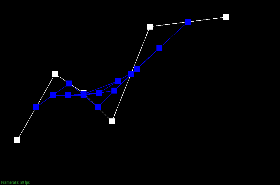
Below, we illustrate running de Casteljau’s algorithm on a Bézier curve with $n=6$ points, going through each step of the process:

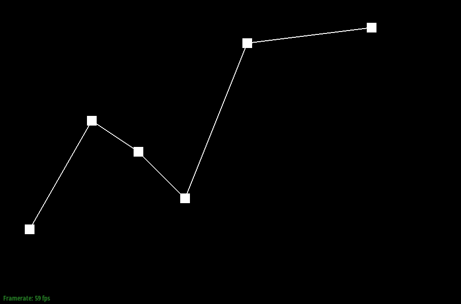Step 0 (Initial Points)	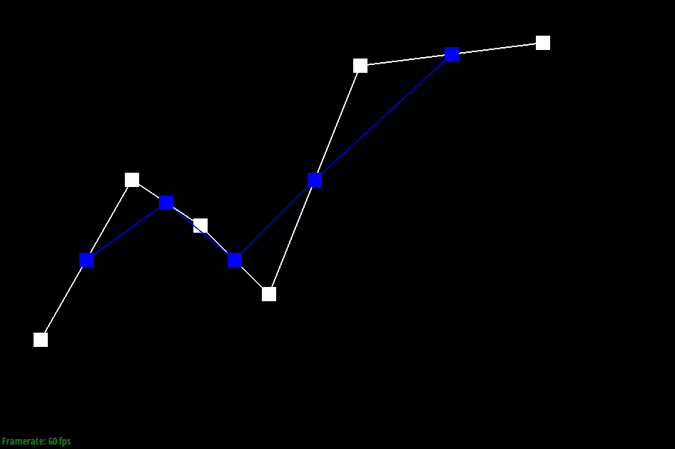Step 1
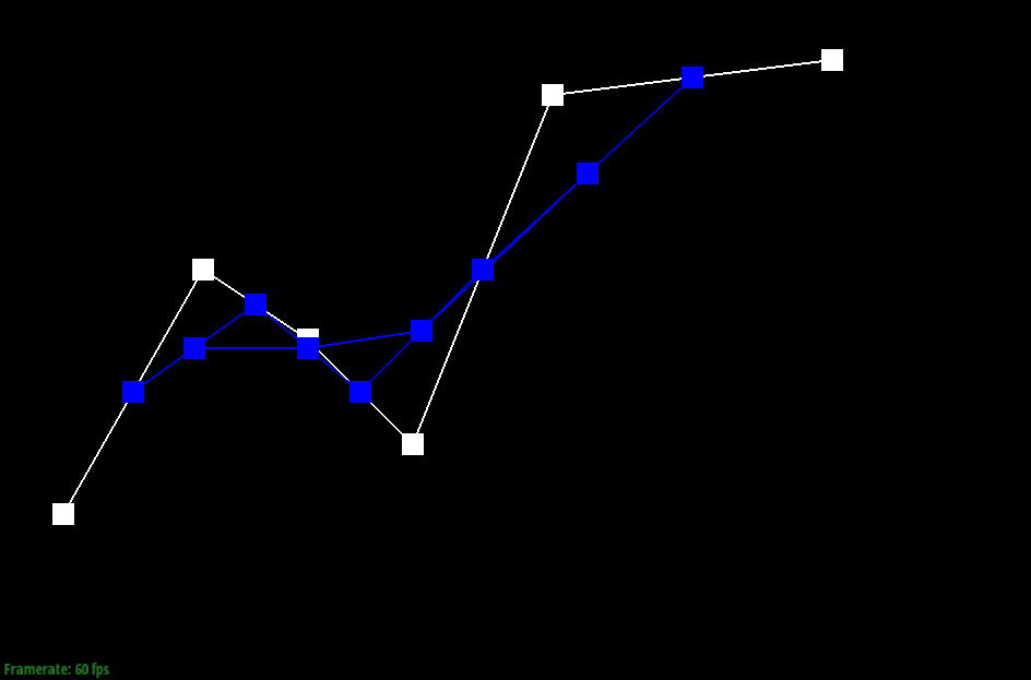Step 2	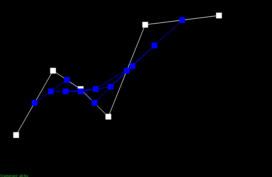Step 3
Step 4	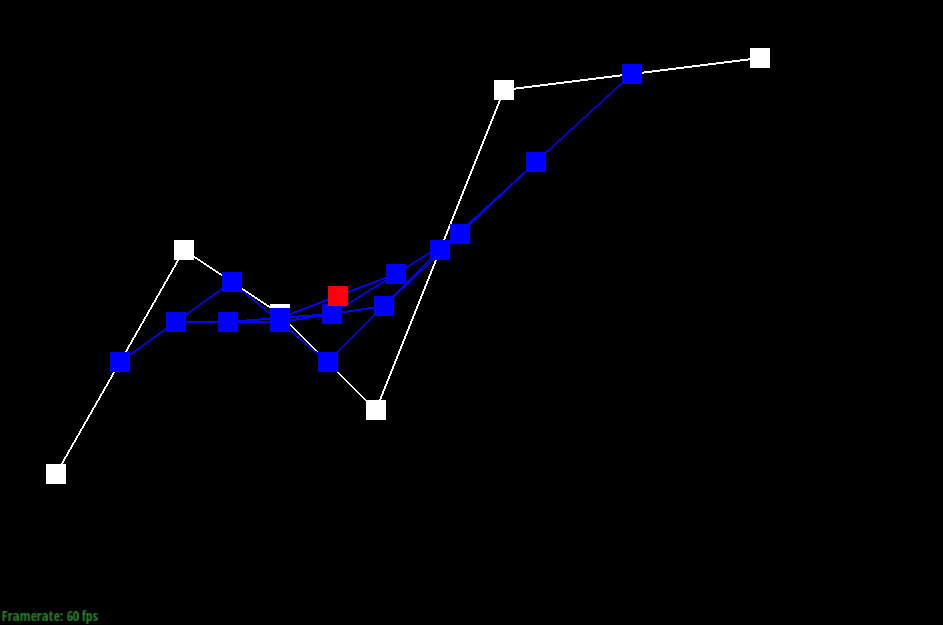Step 5 (Final Point)

And below, we see the final result with the evaluated Bézier curve being displayed as well:

And below, we also modify the parameter $t$ and move around some of the control points, illustrating how it impacts the generated curve:

Bézier Surfaces with Separable 1D de Casteljau

In this part, we will extend de Casteljau’s algorithm from the previous part to handle surfaces as well. Before, we had a single parameter $t$; however, in order to create Bézier surfaces, we will perform the algorithm in two dimensions, have two separate interpolation parameters $u, v$.

The idea for this extension is we first apply our algorithm in one dimension using the parameter $u$, yielding us a set of points. Then, we run the algorithm again in these points, using our other parameter $v$ instead.

Running this on teapot.bez yields us the following result:

Area-Weighted Vertex Normals

For this next part, we implement area-weighted vertex normals — the reason we want to implement this is that these vertex normals are used by Phong shading, which provides better shading than the simple flat shading method.

With this in mind, we implement area-weighted vertex normals by starting with a halfedge. Then, with this halfedge, we get the appropriate face corresponding to it, and iterate through it to get our three vertices $v_0, v_1, v_2$. By subtracting $v_1 - v_0$ and $v_2 - v_0$, we generate edges $e_1, e_2$ which allows us to calculate the normal for this face. Weighting this normal by the area of our face, and then iterating through all the faces, we sum up all of these vertex normals and normalise at the end to obtain the unit normal.

The result of our implementation is shown below:

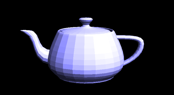Flat Shading	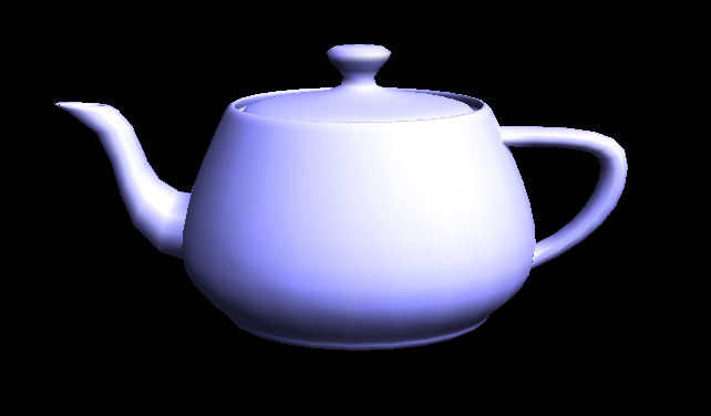Phong Shading

Edge Flip

In this part, we have to implement edge flipping.

As part of our algorithm, we have to reassign all of the different informations (such as the halfedges and their neighbour, vertices, etc.) so that it correctly represents the new configuration after flipping.

To do this, we first identify the corresponding halfedges and their vertices, edges, and faces. From here, using the setNeighbors() function, we update the edges so that they correspond to how they are after the flip operation. And from here, we update the halfedge pointers of the vertices, edges, and faces appropriately.

Below, we illustrate the result of edge flipping a cube:

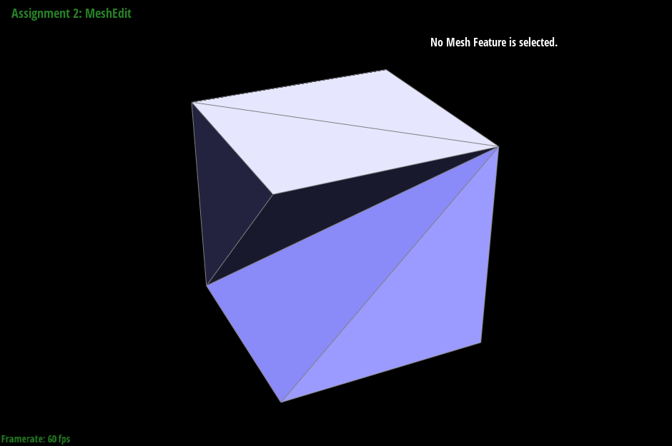No Edge Flips	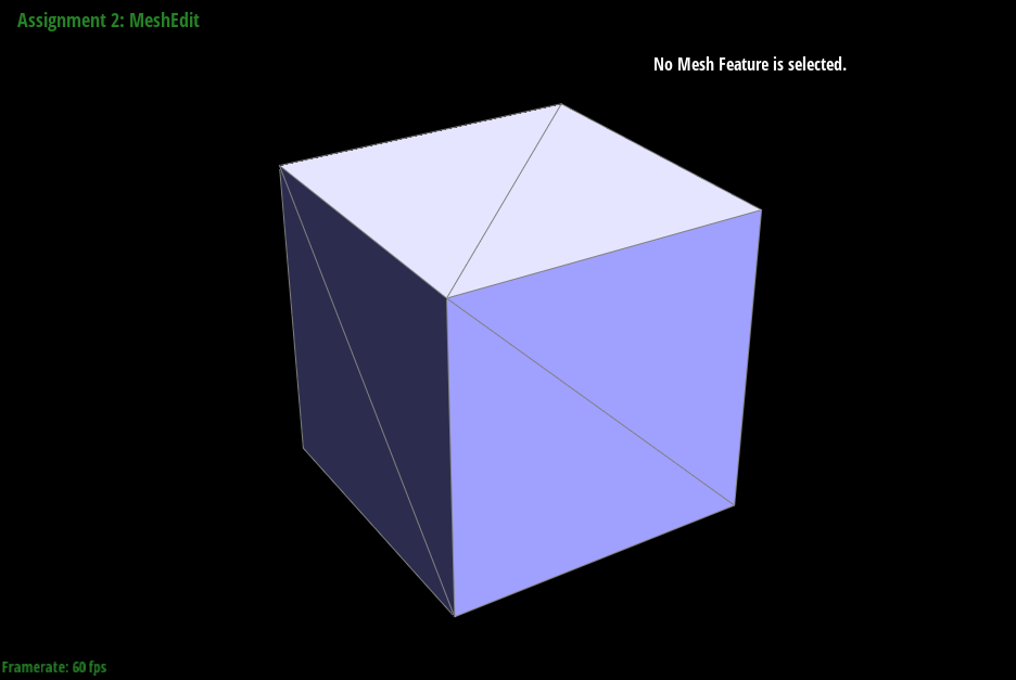Edge Flips

Edge Split

In this part, we implement the Edge Split operation.

Our algorithm is somewhat similar to that of the previous part in terms of having to keep track of all of the different halfedges, vertices, edges, etc. However, since in here, we are splitting an edge up, we will have to introduce new halfedges, faces, etc. to accomodate this change using newHalfedge() and other appropriate functions. And from here, we have to update using setNeighbors() accordingly.

Below is the result of splitting and flipping edges:

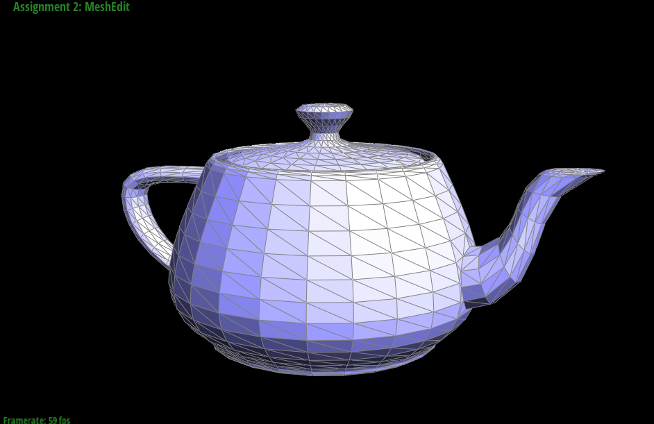Original Teapot	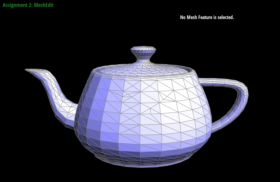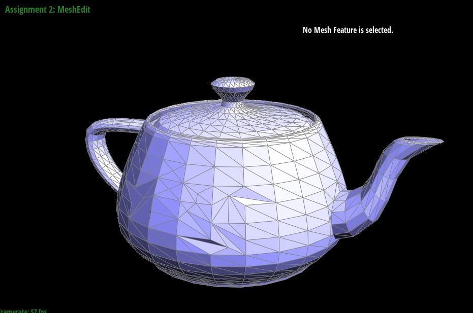Edge Flips and Edge Splits